Introduction

Hi there! I am Xi, a freelancer software engineer in Finland.

My LinkedIn, Github

How to read

I love reading with a dark color theme. You can change themes by clicking the paint brush icon () in the top-left menu bar.

Need to find something specific? Press the search icon () or hit the S key on the keyboard to open an input box. As you type, matching content appears instantly.

Thanks for your time!

AI & Machine Learning

Most new threads land directly in the sidebar first.

When that list gets too long, older threads move into yearly archive pages such as Archive 2026.

This keeps the sidebar recent-first without burying older posts.

What I Learned Trying to Run LTX-Video 2.3 on Apple Silicon

I wanted to learn video generation, picked the fp8 version of Sulphur 2 Base because it looked like it would fit in RAM, downloaded and set up nearly 80GB of files, and then found out it would not run on my Mac Mini M4 Pro with 64GB of RAM.

TypeError: Trying to convert Float8_e4m3fn to the MPS backend
but it does not have support for that dtype.

I did not understand the error at first. The code agent had to explain what the message was really telling me. The answer was not encouraging: there was no practical way to make this setup work on my Mac Mini in its current form. But I learned something new from the failure, and that is what I am writing down here.

The Error

At first, that meant nothing to me. Once I dug into it, the message became clear.

The problem was not memory, the workflow, or a missing node. The backend itself could not handle the datatype the model was stored in.

That changed the investigation.

What I Dug Into

I had to separate three things that are easy to blur together:

1. file size
2. memory pressure
3. backend support

The smaller file was what misled me.

fp8 means each model weight uses 8 bits instead of 16. That matters because the model should need less RAM to load and run. The model file is smaller on disk too, but RAM was the part I cared about.

At first glance, that looked like the whole story. The code agent told me fp8 should be suitable, with only a small quality drop compared with bf16. So I assumed this smaller model version would be the right fit for my Mac Mini.

Not quite.

Apple’s GPU path goes through MPS, Metal Performance Shaders. PyTorch uses that backend to talk to the GPU. And MPS does not support Float8_e4m3fn, the fp8 dtype this model uses.

So the real blocker was not “can I fit this model in RAM?” The real blocker was “can this backend even execute this dtype?” In this setup, the answer was no.

That is a much more useful lesson than a generic “it did not run.”

Why Llama.cpp Feels Different

This also explained something else.

Why can I run quantized LLMs on a Mac, but this video model falls over instantly?

Because the stack is different.

When I run local LLMs with llama.cpp, I am usually using a converted GGUF file, not the original PyTorch model file.

GGUF is the packaging format used by llama.cpp. It stores the model weights, tokenizer metadata, architecture details, and the quantization format in one file. The model might be Q4_K_M, Q5_K_M, or Q8_0.

That last one is easy to misread. Q8_0 is an 8-bit GGUF quantization format. It stores weights as compact integer-like values with scale factors. It is not the same thing as PyTorch Float8_e4m3fn, the fp8 dtype this LTX model uses.

Same 8 bits. Different meaning.

llama.cpp works on Apple Silicon because its GGUF model files, quantized weight formats, scale factors, and Metal kernels are designed to work together. It uses a different path from the PyTorch MPS fp8 path that failed here.

Video generation has another problem: it is a diffusion model.

That means it starts from noise and repeatedly denoises toward frames that match the prompt. Each step depends on the previous one. Small numeric errors can accumulate into visible artifacts: flicker, mushy detail, broken motion, or frames that drift away from each other.

Text models can often tolerate aggressive weight quantization. Video diffusion has less room for that kind of error. Quality is the output.

With LTX, I was asking PyTorch MPS to execute an fp8 model path it does not support. The model never reached a point where I could trade quality for memory or speed. It failed at the dtype boundary.

So “LLMs run on Mac” does not automatically mean “large video models run on Mac too.”

That assumption did not survive contact with reality.

The Practical Takeaway

On Mac, compatibility is not just about how much RAM you have. It is about whether the vendor, hardware, runtime, and model format line up.

On CUDA with NVIDIA H100-class hardware, fp8 is a supported compute path. The hardware has FP8 Tensor Cores, and the software stack is built around that feature. Raw fp8 model in, supported fp8 execution path out.

On this 64GB Apple Silicon machine, fp8 looked like the right size. But size was not enough. The backend could not execute the dtype, so the model format I was holding was not actually runnable in this stack.

After all this, the next version I would try is something like Sulphur 2 Base GGUF. That is closer to the practical path: a quantized model file made for this model family, plus a runtime that knows how to execute that format on Apple Silicon.

The open question is quality. GGUF versions use Q formats, quantized weights, instead of the fp8 float format I tried first. That does not automatically mean the output will look bad. Large diffusion models may tolerate quantization better than I expected.

Because this machine has 64GB of RAM, I would start with Q8_0 if it loads. If it is too slow or too memory-heavy, I would step down to Q6_K, then Q5_K_M, then Q4_K_M.

The real test is visual: same prompt, same resolution, same frame count, same seed. Then compare Q8_0, Q6_K, and Q4_K_M side by side.

Build a Minimal LLM Code Agent: From Loop to Harness

“You can outsource thinking, but not understanding.” - Andrej Karpathy

You’ve heard “code agent” and “harness” a hundred times this year, but do you know how it works? Could you build it in code?

Most people can’t. The words are borrowed, not earned.

This article earns them. We build a minimal LLM code agent from scratch in TypeScript, step by step. By the end, you won’t just know the vocabulary. You’ll know the skeleton underneath it.

The code is built in 30 minutes. The understanding takes the whole article. That’s the point.

TLDR: A code agent is a loop. The loop calls a model, runs tools, and repeats until done. What makes it production-ready is the harness around it: boundaries for tools, context, memory, permissions, and validation. This article builds both from scratch, in TypeScript, milestone by milestone. Source code: minimal-agent.

Milestone 1: The Loop

Strip everything away. What is a code agent at its core?

A loop in runAgent(). That’s it.

import OpenAI from "openai";

const client = new OpenAI({
  baseURL: process.env.OPENAI_BASE_URL ?? "https://api.openai.com/v1",
  apiKey: process.env.OPENAI_API_KEY ?? "none",
});

const MODEL = process.env.MODEL ?? "gpt-4o-mini";

async function runAgent(task: string) {
  const messages: OpenAI.ChatCompletionMessageParam[] = [
    { role: "user", content: task },
  ];

  console.log(`user: ${task}`);

  for (let step = 0; step < 5; step++) {
    console.log(`\n── step ${step + 1}`);

    // action 1;
    const response = await client.chat.completions.create({
      model: MODEL,
      messages,
    });

    // action 2;
    const message = response.choices[0].message;
    messages.push(message);

    // strip <think>...</think> blocks for display only
    const display = message.content
      ?.replace(/<think>[\s\S]*?<\/think>/g, "")
      .trim();
    console.log("model:", display);

    // action 3;
    if (response.choices[0].finish_reason === "stop") {
      return message.content;
    }
  }

  return "Stopped: step limit reached.";
}

const task =
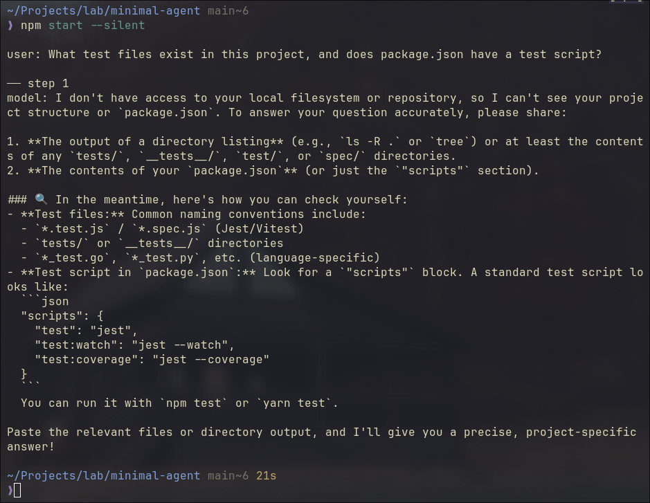
  "What test files exist in this project, and does package.json have a test script?";

runAgent(task);

It sends this exact task to the code agent, "What test files exist in this project, and does package.json have a test script?", then calls runAgent(task) to start the loop.

Three things happen in each iteration:

1. action 1: call the model with the current message history
2. action 2: push the reply into history, print a cleaned version to the terminal
3. action 3: if the model is done, return; if not, loop

flowchart TD
    A([User Task]) --> B[Call Model]
    B --> C[Push Reply to History]
    C --> D{finish_reason = stop?}
    D -- yes --> E([Return Answer])
    D -- no --> F{step < 5?}
    F -- yes --> B
    F -- no --> G([Stopped])

The code above is not pseudocode. You can run it. I run against a local Qwen3.6 35B LLM, but any openai API compatible ones would go, such as gpt-4o-mini with your openai API key.

Several subtle details worth mentioning:

The task hints the model toward tools like list_files and read_file. But none are defined yet. So the model reasons from its own knowledge, does its best, and signals stop after one single step. No looping. Not yet. This is how ChatGPT browser version works.

finish_reason in action 3 isn’t always "stop". "length" means output hit the token limit, cut off mid-thought. "content_filter" means it was blocked. Production handles all of them explicitly. In this demo, we assume it’s always the happy path.

That step < 5 guard is not cosmetic. A confused model won’t stop itself. The step limit is the first harness piece, already baked in.

Milestone 2: Tools

Now give it eyes (tools).

Tools are not system prompt tricks. They’re a structured contract. The code agent passes a list of tool definitions alongside your messages. The model reads the descriptions and decides which one to call.

// ... imports, client, MODEL same as before

// ── Tool definitions (what the model sees)
const tools: OpenAI.ChatCompletionTool[] = [
  {
    type: "function",
    function: {
      name: "list_files",
      description: "List files and directories at a given path.",
      parameters: {
        type: "object",
        properties: {
          path: { type: "string", description: "Directory path to list." },
        },
        required: ["path"],
      },
    },
  },
  {
    type: "function",
    function: {
      name: "read_file",
      description: "Read the contents of a file.",
      parameters: {
        type: "object",
        properties: {
          path: { type: "string", description: "File path to read." },
        },
        required: ["path"],
      },
    },
  },
];

// ── Tool implementations (what actually runs)
function list_files(filePath: string): string {
  const entries = fs.readdirSync(filePath, { withFileTypes: true });
  return entries
    .map((e) => (e.isDirectory() ? `${e.name}/` : e.name))
    .join("\n");
}

function read_file(filePath: string): string {
  return fs.readFileSync(filePath, "utf-8");
}

function runTool(name: string, args: Record<string, string>): string {
  if (name === "list_files") return list_files(args.path);
  if (name === "read_file") return read_file(args.path);
  return `Unknown tool: ${name}`;
}

// ── Agent loop
async function runAgent(task: string) {
  // ... messages setup same as before
  for (let step = 0; step < 5; step++) {
    const response = await client.chat.completions.create({
      model: MODEL,
      messages,
      tools, // <-- added
    });

    const message = response.choices[0].message;
    messages.push(message);

    if (response.choices[0].finish_reason === "tool_calls") {
      const toolCall = message.tool_calls![0];
      const args = JSON.parse(toolCall.function.arguments);
      const observation = runTool(toolCall.function.name, args);
      messages.push({
        role: "tool",
        tool_call_id: toolCall.id,
        content: observation,
      });
    } else {
      // ... print and return same as before
    }
  }
}

// ... task and runAgent(task) same as before

Think about how you’d solve this yourself.

You’d list the files first to get your bearings. Then open the specific file you need.

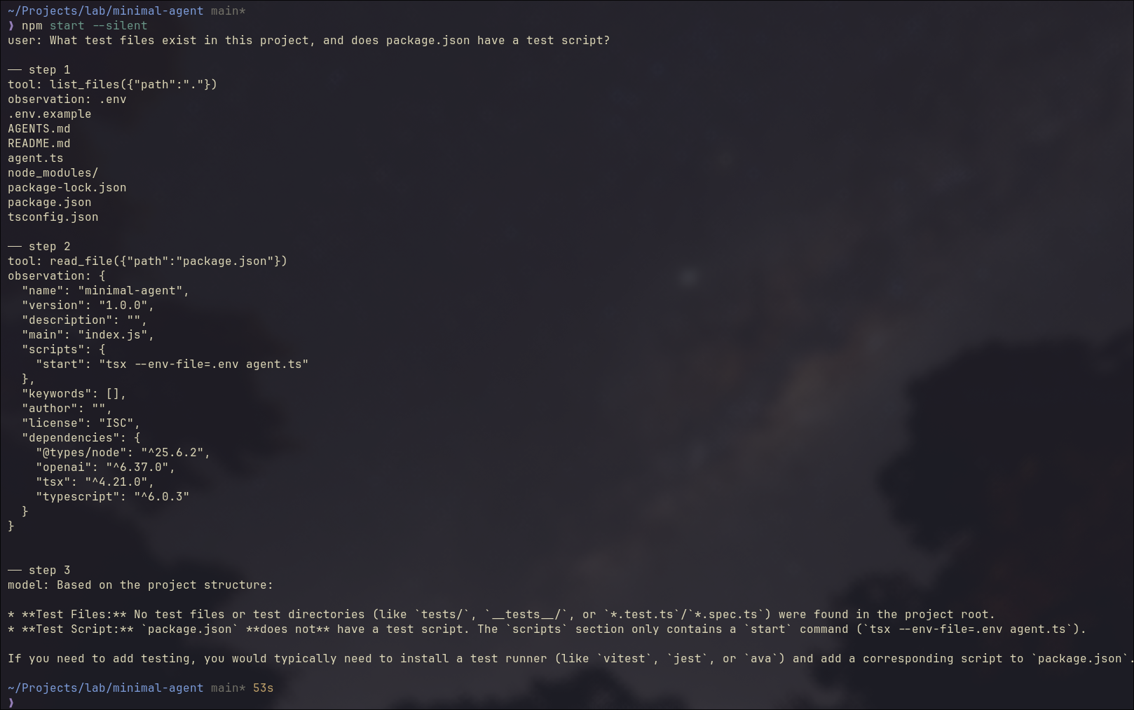
The model does the same. It calls list_files("."), scans the result, then calls read_file("package.json"). Two steps. Then it has what it needs and signals stop.

The diagram shows exactly that.

sequenceDiagram
    participant Tool
    participant Agent
    participant Model

    Agent->>Model: messages
    Model-->>Agent: tool_calls
    Agent->>Tool: list_files(".")
    Tool-->>Agent: response
    Agent->>Model: messages + observation
    Model-->>Agent: tool_calls
    Agent->>Tool: read_file("package.json")
    Tool-->>Agent: response
    Agent->>Model: messages + observation
    Model-->>Agent: stop
    Agent->>Agent: done

The code running result is in the screenshot below:

Steps 1 and 2 follow the same pattern: the model requests a tool call, the agent runs it and sends the observation back.

Step 3 is different. No tool call. The model has enough context now and answers directly. That’s the stop signal, and the final answer prints.

Think of tools as sensors in an IoT system. They sample the environment and send readings back. The model, like a controller, makes decisions based on what it receives.

Feed it accurate readings, it reasons correctly. Feed it wrong ones, it reasons confidently in the wrong direction. The model has no way to tell the difference. It just processes what arrives.

You could return fake data. Wrong file contents. A made-up directory listing. The model would accept it, reason over it, and answer confidently. No verification.

The quality of the agent’s output is only as good as the observations its tools return.

Milestone 3: Tool Boundary

Now add run_command. The model can execute shell commands.

list_files and read_file use Node’s fs module. You’re calling well-defined Node APIs. Node handles the underlying OS interaction, and the security contract is clearly scoped: read the filesystem, nothing else.

run_command is different. It hands a string to the shell and lets the shell decide what happens. No guardrails. Any binary, any argument, any side effect. That’s a different layer entirely, and it needs a different trust model.

// ... imports, client, MODEL, tools, list_files, read_file, runAgent same as before

const ALLOWED_COMMANDS = ["ls", "cat", "echo", "node", "npm", "rg"];

function run_command(command: string): string {
  const binary = command.trim().split(/\s+/)[0];
  if (!ALLOWED_COMMANDS.includes(binary)) {
    return `Error: '${binary}' is not an allowed command.`;
  }
  return execSync(command, { encoding: "utf-8" });
}

const task =
  "List the files in this directory, read package.json, and run `node --version`.";

runAgent(task);

Notice the whitelist? It is the guardrail we build. The model can reach the shell, but only through these specific doors. If we send the task to run rm AGENTS.md, agent would refuse it as below.

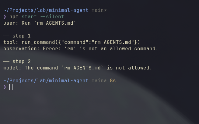
The code run above has the task: “Run rm AGENTS.md”, and it has two steps.

Step 1: the model calls run_command("rm AGENTS.md"). It doesn’t know rm is blocked. The whitelist fires, returns an error string as a normal observation. Step 2: the model reads it and reports back.

Two subtle points I’d like to point out.

First: the model doesn’t build the guardrail. The agent does. The model still tried to run rm, no hesitation, no special awareness. Your code intercepted it. You can’t rely on the model to protect you from itself. The boundary has to live in the harness.

Second: real harnesses return richer observations. Our run_command returns a plain string. Production systems return exit codes, stderr separated from stdout, truncation markers. Without exit codes, the model can’t tell “command ran and produced nothing” from “command failed silently.” Feed it thin observations, it fills the gaps with guesses.

What a Real Agent Needs

The loop is running. It can list files, read files, run commands. The demo works.

But “works in a demo” is not the same as “works on real tasks.” Run this code agent on anything non-trivial and four specific things will break:

1. Context overflows. Long tool observations grow the message array. Hit the token limit, the API throws.
2. No memory. Close the terminal, restart, it knows nothing about your project.
3. Unchecked commands. No confirmation before running something irreversible.
4. False completion. The model says “done.” Nothing was actually written or tested.

These aren’t hypothetical. Each one is a failure mode you will hit. The next four milestones add a boundary for each.

Milestone 4: Context Boundary

Context isn’t just a technical limit. It’s everything the model can see right now.

Transformers don’t attend equally across the context. The model pays more attention near the start and near the end. Bury something in the middle and the model struggles to reach it. The longer the context, the harder the attention. Researchers call this the “lost in the middle” problem.

So the goal isn’t just “stay under the limit.” It’s “keep the right things visible.”

That means three operations: pick what goes in, remove what’s useless, condense what’s redundant. Each is a judgment call. Each is hard. Together, they look a lot like the old embedded discipline: limited RAM, everything competing for it, no room for waste. The constraint is different. The problem shape is the same.

In our demo, we take the simple approach: truncate anything too long.

const raw = await runTool(toolCall.function.name, args);
const observation =
  raw.length > 2000 ? raw.slice(0, 2000) + "\n[...truncated]" : raw;

This is a blunt instrument. It works for a demo. In production, you’d summarize instead: call the model again on just the observation, get a condensed version, push that. Tools like RTK solve this at the CLI layer, compressing the tool call result before it ever reaches the model.

A side note, the screenshot below is my RTK session summary for ~2 week usage. 589 commands run, 392K tokens saved. That’s 46.8% of input tokens eliminated before the model ever saw them.

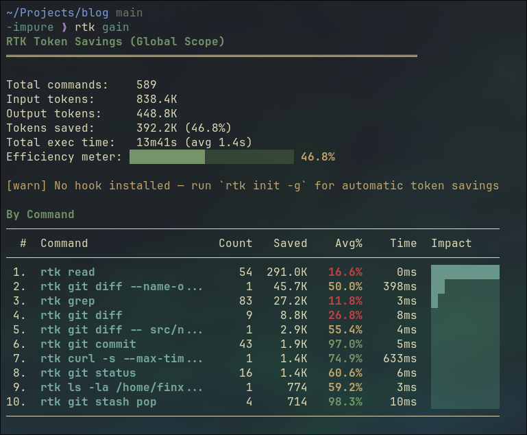
One broader observation worth making here: CLI tools are starting to evolve toward output that code agents can read efficiently. ls returning 200 lines of noise made sense when a human was reading it. When a code agent reads it, that’s wasted tokens. RTK is a shim for the transition period. Long-term, tools will output compact, structured data natively. The same shift happened to APIs when mobile came along.

Milestone 5: Memory Boundary

Context is what’s in the messages array right now. Memory is what survives closing the terminal.

Add an AGENTS.md to the project root:

# Project Rules

Always respond in Simplified Chinese (简体中文).

Load it as a system message at startup:

function loadMemory(): OpenAI.ChatCompletionMessageParam[] {
  try {
    const rules = fs.readFileSync("AGENTS.md", "utf-8");
    return [{ role: "system", content: rules }];
  } catch {
    return [];
  }
}

const messages = [...loadMemory(), { role: "user", content: task }];

Run the same task as before. The model now responds in Chinese. Delete AGENTS.md, run again: English. The difference is visible in one line.

Trust me, those are proper Chinese. The agent isn’t broken. 😄

Continuity across sessions.

For personal agents, memory isn’t a feature. It’s the whole point. Projects like OpenClaw and Hermes are built around this: an assistant that knows your preferences, your history, your context. Context is temporary. Memory is what makes it yours.

Which is why memory management is the harder problem. Context management asks: what should the model see right now? Memory management asks: what’s worth keeping at all? What to store. What to discard. When to surface it. How to retrieve the right piece without loading everything.

Nobody has fully solved this. It’s one of the most active areas in agent research. Some draw the parallel to human sleep: one leading theory holds that sleep is when the brain consolidates the day’s experiences, strengthening useful patterns and discarding the rest. We don’t yet have that for LLMs. The framing is the same. The solution isn’t.

Milestone 6: Permission Boundary

run_command has a whitelist. That’s the outer gate. But some commands in the whitelist are still risky. npm install, npm run build — these change state.

Add a second tier: commands that require confirmation before running.

const AUTO_COMMANDS = ["ls", "cat", "echo", "node", "rg"];
const CONFIRM_COMMANDS = ["npm"];

async function run_command(command: string): Promise<string> {
  const binary = command.trim().split(/\s+/)[0];
  if (!AUTO_COMMANDS.includes(binary) && !CONFIRM_COMMANDS.includes(binary)) {
    return `Error: '${binary}' is not an allowed command.`;
  }
  if (CONFIRM_COMMANDS.includes(binary)) {
    const approved = await ask(`Allow: ${command} ? (y/n) `);
    if (!approved) return "User denied the command.";
  }
  return execSync(command, { encoding: "utf-8" });
}

Three tiers: auto, confirm, deny. The model doesn’t know which tier a command is in. It just calls the tool. Your code decides what happens next.

This is the same design Claude Code uses. Anthropic documented the tension: ask for every write and run command, and users get approval fatigue. Never ask, and you amplify risk. Their production answer involves a classifier that identifies truly risky actions. Our demo answer is a simple tier list. The principle is identical: the permission boundary keeps the model from being the last line of defense.

Milestone 7: Write and Validate

A code agent that can only read and run is half an agent. It can answer questions. It can’t produce things. Add write_file.

function write_file(filePath: string, content: string): string {
  fs.writeFileSync(filePath, content, "utf-8");
  return `Written: ${filePath}`;
}

The signal is simple: the tool returns on success, throws on failure. "Written: summary.txt" means it worked. The loop closes. That’s the first layer of validation: the agent knows the write succeeded.

The second layer runs after the agent finishes. Check independently.

runAgent(task).then(() => {
  const ok =
    fs.existsSync("summary.txt") &&
    fs.readFileSync("summary.txt", "utf-8").trim().length > 0;
  console.log(
    ok
      ? "\nValidation passed: summary.txt written."
      : "\nValidation failed: summary.txt missing or empty.",
  );
});

Two tiers. The tool return closes the inner loop. The external check closes the outer one. “Done” is not a feeling. It’s evidence.

Models are excellent at sounding confident. That confidence has no relationship to whether the work was actually done. Traditional CI fails loudly with logs. A code agent can succeed quietly and lie. Both checks are what makes completion mean something.

How do Claude Code and Codex handle this on longer tasks? Same principle at scale: check exit codes, run the test suite, read back files they just wrote. Claude Code’s Todo system marks tasks complete only after the environment confirms, not after the model claims. The exact mechanisms for complex multi-step recovery are still an active area.

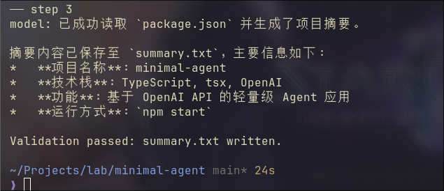
This is the final version of the demo. Let’s run it.

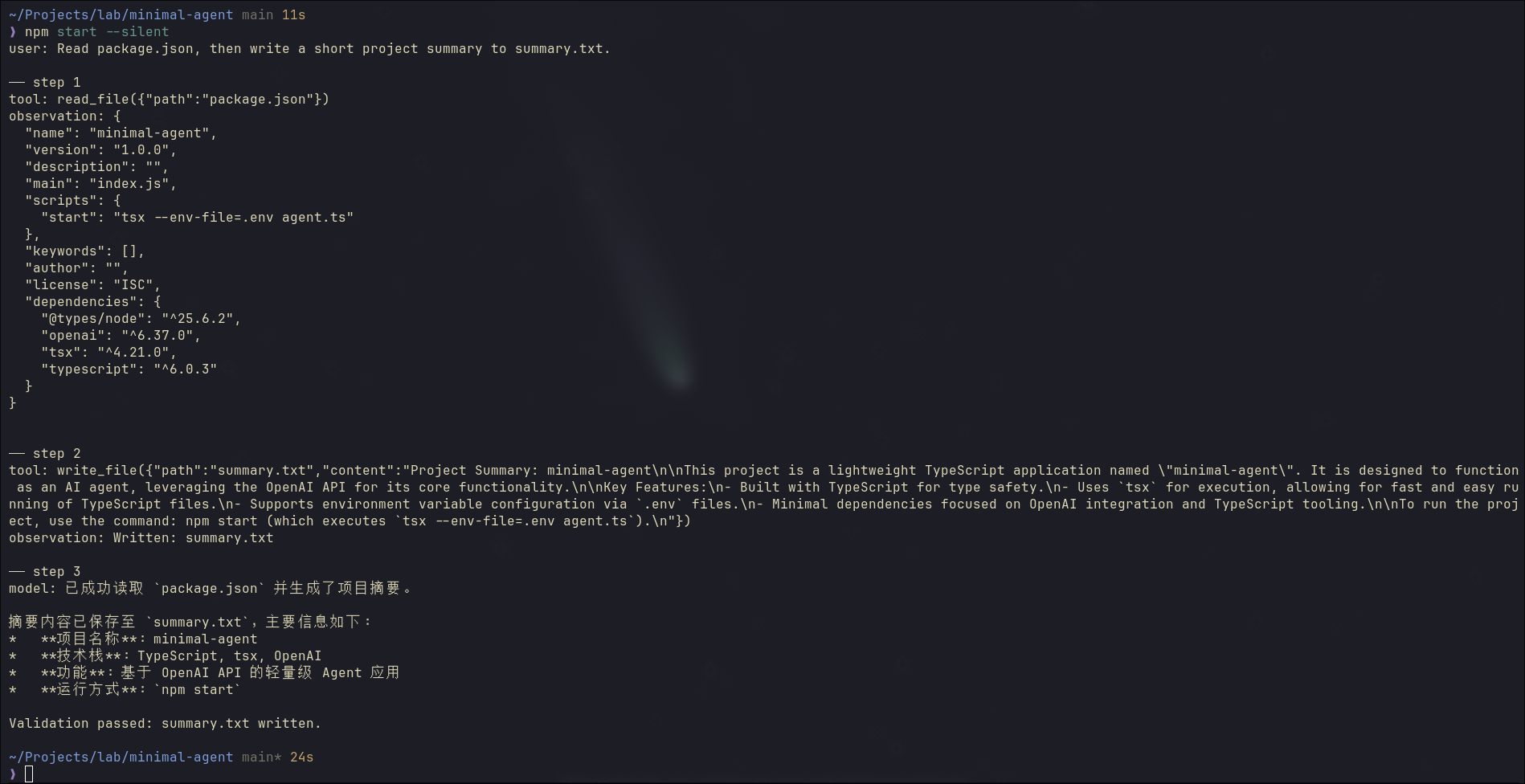
The agent reads package.json, writes the summary to summary.txt in English, then responds in Chinese (AGENTS.md is still loaded). The external check confirms the file is written. Read, write, memory, validation: the full harness, working together.

The Model Inside the Loop

The harness is fixed while we can swap the model like OpenCode and pi do.

Qwen3.6 35B I use chains tools correctly, recovers from failures, and produces useful output. A weak 1B model hallucinates file paths, stops after one tool call, or returns empty content.

That’s the separation this demo was built to show, and honestly it’s the thing I find most clarifying about building this yourself. The model defines the ceiling: how far it can reason, how well it recovers, how much ambiguity it can handle. The agent defines the floor: what’s allowed, what gets checked, what can’t go wrong even if the model tries.

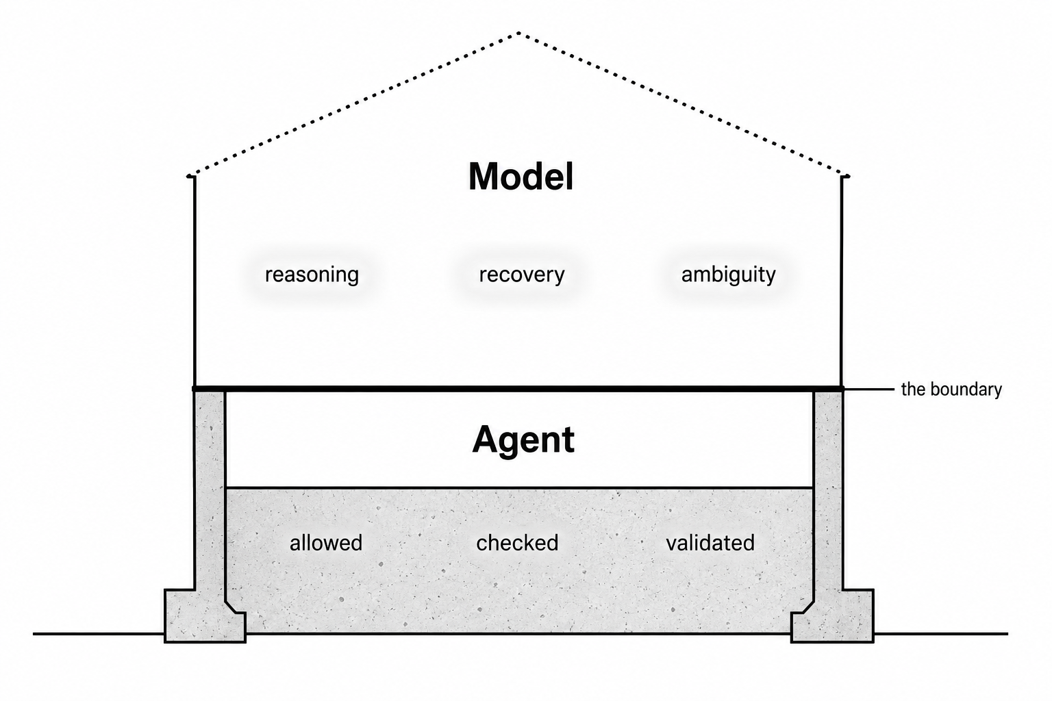
You can’t train the expensive model. But you can build the code agent. The harness is just code. That boundary is worth holding onto.

Wrap Up

Look at what we built:

flowchart LR
    subgraph Minimal["Minimal Code Agent"]
        L([Loop])
    end

    subgraph Harness["Harness"]
        TB[Tool Boundary] --> L
        CB[Context Management] --> L
        MB[Memory Boundary] --> L
        PB[Permission Boundary] --> L
        VB[Validation Boundary] --> L
    end

Claude Code is this. Codex is this. Every serious code agent framework is this. The loop is always simple. The work is always in the boundaries.

Build it yourself. Feel each piece land. Then when someone says “Claude Code uses a harness layer,” you won’t nod along. You’ll know exactly what they mean.

That’s the understanding Karpathy was talking about. You can’t outsource it.

Source code: minimal-agent.

Salesforce Headless 360: Agent-First or Just Hype?

User agents are multiplying. Quietly. Everywhere.

Claude books meetings. Copilot writes code. Support tickets close without anyone opening a browser.

This is why Salesforce announced Headless 360. Not to improve the existing platform. To survive what’s coming.

Because this isn’t A to A+. It’s A dying and an unprecedented B appearing. In Salesforce, A is the no/low-code GUI. B is the user agent.

That distinction is why this article exists.

To understand why, go back to the 1950s.

The shipping container didn’t make dockworkers more efficient. It made them unnecessary.

Before containers: armies of workers, every cargo type handled by hand, every port built around human labor.

Then containers came, and the entire logic of moving cargo had to be rethought from the ground up. The work didn’t get faster. The work disappeared. Break-bulk was gone. London’s docks emptied. New York’s piers went silent. Felixstowe and Port Newark rose in their place. Built for a machine, not a hand.

That’s not A to A+. That’s A dying. B appearing. Entirely different rules.

AI is doing the same thing to knowledge work. Removing the human from the loop entirely, for entire categories of work.

This wave also moves faster than any before it. Smartphones took four years. iPhone launched in 2007. By 2011, crossed 50% in major markets.

Enterprise software moves faster. No hardware to buy. Buyers have budget authority. The pressure is headcount, not adoption friction.

If 2026 is year zero, 2028 is not a stretch.

Salesforce’s Headless 360 is doing the same thing to the GUI-first paradigm.

The old world isn’t gone (yet). But it’s no longer where the platform is heading.

Old world:

graph LR
    Human[Human] --> GUI[GUI]
    GUI --> Platform[Platform]

New world:

graph LR
    Human[Human] --> UserAgent[User Agent]
    UserAgent --> PlatformInterface[Platform Interface]
    PlatformAgent[Platform Agent] -.->|Supervises| PlatformInterface

But a user agent isn’t just a faster human clicking buttons. It’s a different beast entirely.

It doesn’t browse. It calls APIs directly, moves through multi-step sequences without pausing, and never waits for a screen to load. No GUI to confirm. No human in the loop to catch a wrong turn.

You’ve been there. An agent tells you to go to a link, click a button in the top right, then do this, then do that. Not because the agent wants to. Because the platform doesn’t support headless interaction.

My simple rule:

If you remove all the GUI, the agent should still be able to do the same work. If it can’t, the platform isn’t agent-first.

A user agent reasons through multi-step sequences on its own. It carries context across every action. It decides, executes, and moves on. Platforms were never built for any of that.

A new beast needs a new foundation. Two things make or break it:

Semantics.

Agents can’t guess intent. They have no visual cues, no hover states, no tooltips. Without machine-readable context, they hallucinate paths, retry blind, and trigger side effects no one planned for.

Many platforms ship CLIs, APIs, MCPs, and skills. They call it “agent-first”. It’s an important step. But it’s missing the soul.

The soul is semantics.

A good CLI doesn’t just expose commands. It tells agents what to expect:

• --help with clear, structured output
• --dry-run for any action with side effects
• --json for machine-readable responses
• Clean stdout, stderr, and exit codes
• Good examples. LLMs love examples.

APIs follow the same logic. The interface and the meaning.

• Schema descriptions that explain intent, not just structure
• Reversibility signals. Agents can’t read warning modals.
• Structured errors: retry, escalate, or abort
• Idempotency keys. Agents retry. Without them, retries create duplicates.

MCP servers should expose a minimal contract. Not everything at once. Let the agent explore when it needs to. Fewer tools visible = less noise = sharper decisions.

Agent skills are different. Each feature gets its own skill. For example, a user agent needs to create a flow. It finds the flow creating skill via llms.txt. Reads the contract: inputs, outputs, side effects. Knows exactly what format to pass. No guessing. No docs to scrape.

flowchart LR
    UA[User Agent] -->|discover| L[llms.txt]
    L -->|find skill| S[Skill Contract]
    S -->|read contract| UA
    UA -->|execute| A[Action]

The goal isn’t coverage. It’s clarity.

Observability.

Agents don’t interact with the platform like humans. They interact constantly. Thousands of actions where a human might take one. That volume demands auditing and logging at a scale no human admin can process.

The data is there. The problem is who reads it. No human can keep up. The platform needs to put agents in the admin role too. Monitoring what’s happening. Flagging anomalies. Catching what no one would catch manually.

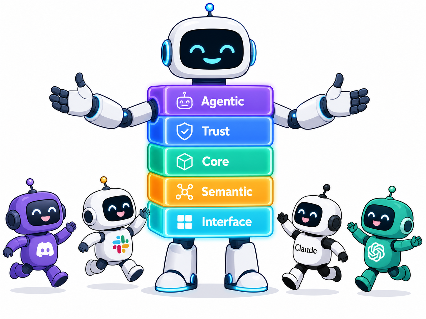
These two challenges shaped how I think about platform design. Five layers.

flowchart LR
    Human[Human] --> UserAgent[User Agent]
    UserAgent --> E
    subgraph E[5 - Agentic Layer]
        direction TB
        A[1 - Interface Layer] --> B[2 - Semantic Layer]
        B --> C[3 - Core Layer]
        C --> D[4 - Trust Layer]
    end

1. Interface Layer

APIs, CLIs, MCPs, skills. The front door that lets user agents enter the platform.

Having an interface isn’t enough. It must be designed for agents, not humans who happen to type commands. Without context, agents guess and hallucinate. That’s what the next layer fixes.

2. Semantic Layer

This is the one everyone skips. Companies think exposing an interface is enough. But an interface without meaning is a trap. Agents guess, retry blind, trigger side effects no one planned for.

Good semantics tell agents what to expect, what’s reversible, what to avoid. The interface and the meaning. That’s what makes an agent reliable, not just capable.

The specifics are covered above, in the CLI, API, MCP, and skills breakdown.

3. Core Layer

The data model, automations, custom business logic. Everything that already exists in the platform and makes it valuable.

This is the moat. Years of customer configuration, flows, Apex, integrations, all locked into Salesforce. That doesn’t disappear. It gets exposed to agents, cleanly, through the Semantic Layer above.

But most orgs are monolithic jungles. A user clicks a button. That invokes Apex, which fires a trigger, which kicks off a flow, which updates another object, which fires another trigger, which waits for approvals, which sends notifications.

The ideal: the core is detangled into composable units. The platform handles the low-level wiring. Agents pick what they need and chain at the right level of abstraction.

The reality: most orgs carry that technical debt. That’s fine, as long as the agent can see the full chain clearly. Not guess it. See it. Then it can act deliberately.

4. Trust Layer

Auditing, logging, error collecting. The platform’s record of everything user agents do.

Most platforms stop at logging. But agents can do something humans never bothered with: submit rich diagnostics when something goes wrong. Exact inputs, the decision path, the error. Not a vague report. A full trace.

For that to work, the platform needs to provide the channel. An API for agents to submit feedback directly. Not passive logs waiting to be scraped. Active submission, by design.

Software doesn’t survive by grand roadmaps. It survives by evolving toward what users actually need, one fix at a time. Agents generate the richest signal of what’s failing and what matters. That trace is gold.

5. Agentic Layer

This layer sits on top of everything else. It’s the platform watching itself.

Agents that monitor incoming actions, track performance, run A/B tests, roll back automatically.

These are the admins of the new world. Not replacements for human admins. They handle the scale and speed no human can.

Diagnostic data arrives. They find the pattern. They trigger the fix. A new API version ships. They test, score, and roll back if needed. No delay.

Wrap Up

The Semantic Layer and the Trust Layer are unlike anything the platform has built before. And they’re the easiest to ignore.

Salesforce built its empire on CRM data and the GUI-first strategy. The data and the trust it carries remain the brand. The GUI-first paradigm on top of it is fading. Some adapt and thrive. Others become relics.

Salesforce Headless 360 is a good move. But the vision is not enough. The implementation is the key. The real work is in the layers.

Classification

Comparing to regression (predict values), classification has more areas to pay attention to.

In regression, the prediction target is a continuous value, and a single error metric often gives a decent first signal.
In classification, model quality depends on decision boundaries, class balance, and threshold choices, so evaluation is usually the hard part.
This thread uses MNIST to show not only how to train classifiers, but how to reason about whether their predictions are trustworthy.

1) MNIST dataset

MNIST is used because it’s:

• easy to visualize,
• large enough to see realistic evaluation issues,
• naturally supports binary, multiclass, and beyond.

Why this code matters: We start with a controlled dataset so you can focus on evaluation logic instead of data cleaning noise.
What to look for: The train/test split and shuffling are critical; without these, later metrics can be misleading.
Common trap: Treating this split pattern as universal. In production, prefer stratified split and time-aware split when data is temporal.

import numpy as np
import matplotlib.pyplot as plt
from sklearn.datasets import fetch_openml

mnist = fetch_openml("mnist_784", as_frame=False)
X, y = mnist.data, mnist.target.astype(np.uint8)

X_train, X_test = X[:60000], X[60000:]
y_train, y_test = y[:60000], y[60000:]

shuffle_idx = np.random.permutation(60000)
X_train, y_train = X_train[shuffle_idx], y_train[shuffle_idx]

def plot_digit(image_data):
    image = image_data.reshape(28, 28)
    plt.imshow(image, cmap="binary")
    plt.axis("off")

plot_digit(X[0])
plt.show()

2) Training a binary classifier (a “5-detector”)

• positive class: “is digit 5”
• negative class: “not 5”

Why this code matters: Binary classification is the simplest setting to learn precision/recall trade-offs.
What to look for: decision_function gives a score for ranking confidence, while predict applies a default threshold to return True/False.
Common trap: Reading decision scores as probabilities. They are margin-like scores, not calibrated probabilities.

from sklearn.linear_model import SGDClassifier

y_train_5 = (y_train == 5)
y_test_5 = (y_test == 5)

sgd_clf = SGDClassifier(random_state=42)
sgd_clf.fit(X_train, y_train_5)

some_digit = X[0]
print("Prediction:", sgd_clf.predict([some_digit]))
print("Decision score:", sgd_clf.decision_function([some_digit]))

3) Performance measures: why accuracy can lie

Why this code matters: If only ~10% of images are digit 5, a naive model can get high accuracy by mostly predicting “not 5.”
What to look for: Compare SGD accuracy against DummyClassifier baseline. If they are close, your model may not be useful.
Common trap: Celebrating high accuracy without checking class distribution or baseline performance.

from sklearn.model_selection import cross_val_score
from sklearn.dummy import DummyClassifier

print("SGD accuracy:",
      cross_val_score(sgd_clf, X_train, y_train_5, cv=3, scoring="accuracy"))

dummy_clf = DummyClassifier(strategy="most_frequent")
print("Dummy accuracy:",
      cross_val_score(dummy_clf, X_train, y_train_5, cv=3, scoring="accuracy"))

4) Confusion matrix

Why this code matters: The confusion matrix is the source of truth behind most classification metrics.
What to look for:
TN: correctly rejected non-5s, FP: wrongly flagged non-5s as 5, FN: missed real 5s, TP: correctly found 5s.
Common trap: Looking only at diagonal totals without considering whether FP or FN is more costly in your use case.

from sklearn.model_selection import cross_val_predict
from sklearn.metrics import confusion_matrix

y_train_pred = cross_val_predict(sgd_clf, X_train, y_train_5, cv=3)
confusion_matrix(y_train_5, y_train_pred)

5) Precision, recall, F1

Why this code matters: These metrics let you optimize for the failure mode that matters most.
What to look for:
High precision means fewer false alarms; high recall means fewer misses; F1 balances both when you need a single score.
Common trap: Maximizing F1 by default. In many domains, one error type is far more expensive than the other.

from sklearn.metrics import precision_score, recall_score, f1_score

precision = precision_score(y_train_5, y_train_pred)
recall = recall_score(y_train_5, y_train_pred)
f1 = f1_score(y_train_5, y_train_pred)

precision, recall, f1

6) Precision/Recall trade-off

Why this code matters: Classifiers output scores, and your threshold turns those scores into decisions.
What to look for: As threshold increases, precision usually rises while recall falls. Pick threshold based on product/business cost.
Common trap: Keeping threshold at default 0 without validating if it matches your required precision or recall target.

from sklearn.metrics import precision_recall_curve

y_scores = cross_val_predict(
    sgd_clf, X_train, y_train_5,
    cv=3,
    method="decision_function"
)

precisions, recalls, thresholds = precision_recall_curve(
    y_train_5, y_scores
)

plt.plot(thresholds, precisions[:-1], label="precision")
plt.plot(thresholds, recalls[:-1], label="recall")
plt.legend()
plt.xlabel("threshold")
plt.grid(True)
plt.show()

7) ROC curve

Why this code matters: ROC summarizes ranking performance across all thresholds.
What to look for: Curves closer to top-left and larger AUC indicate better separability than random guessing.
Common trap: Using ROC alone on imbalanced data. Precision-Recall curves are often more informative when positives are rare.

from sklearn.metrics import roc_curve, roc_auc_score

fpr, tpr, roc_thresholds = roc_curve(y_train_5, y_scores)
auc = roc_auc_score(y_train_5, y_scores)

plt.plot(fpr, tpr, label=f"SGD (AUC={auc:.4f})")
plt.plot([0, 1], [0, 1], "--", label="random")
plt.xlabel("FPR")
plt.ylabel("TPR")
plt.legend()
plt.grid(True)
plt.show()

8) Random Forest comparison

Why this code matters: Same task, different model family; this checks whether the issue is data-limited or model-limited.
What to look for: Compare auc (SGD) vs auc_forest. Better AUC suggests better ranking quality over thresholds.
Common trap: Comparing models using different validation setups. Keep CV split and metric consistent for fair comparison.

from sklearn.ensemble import RandomForestClassifier

forest_clf = RandomForestClassifier(random_state=42, n_estimators=200)

y_probas_forest = cross_val_predict(
    forest_clf,
    X_train,
    y_train_5,
    cv=3,
    method="predict_proba"
)

y_scores_forest = y_probas_forest[:, 1]
auc_forest = roc_auc_score(y_train_5, y_scores_forest)

auc, auc_forest

9) Multiclass classification

Why this code matters: Real tasks often require choosing among many labels, not just yes/no.
What to look for: Baseline multiclass accuracy vs scaled-pipeline accuracy; SGD usually benefits from feature scaling.
Common trap: Forgetting to include preprocessing in the cross-validation pipeline, which causes leakage or inconsistent evaluation.

from sklearn.preprocessing import StandardScaler
from sklearn.pipeline import make_pipeline

sgd_clf_multi = SGDClassifier(random_state=42)
print("Multiclass accuracy:",
      cross_val_score(sgd_clf_multi, X_train, y_train,
                      cv=3, scoring="accuracy"))

sgd_scaled = make_pipeline(
    StandardScaler(),
    SGDClassifier(random_state=42, max_iter=100)
)

print("Scaled accuracy:",
      cross_val_score(sgd_scaled, X_train, y_train,
                      cv=3, scoring="accuracy"))

10) Error analysis

Why this code matters: A confusion matrix for multiclass reveals where the model struggles, not just how much.
What to look for: Pairs of digits with high confusion (e.g., similar shapes). Those patterns guide targeted improvements.
Common trap: Stopping at one aggregate score instead of diagnosing specific confusion pairs.

from sklearn.metrics import ConfusionMatrixDisplay

y_train_pred_multi = cross_val_predict(
    sgd_scaled, X_train, y_train, cv=3
)

cm = confusion_matrix(y_train, y_train_pred_multi)
ConfusionMatrixDisplay(cm).plot(cmap="Blues")
plt.show()

11) Multilabel & Multioutput

Multilabel

Why this code matters: One sample can have multiple valid labels (not mutually exclusive), which is common in tagging systems.
What to look for: Output has multiple booleans per sample: here, >=7 and odd are predicted together.
Common trap: Treating multilabel as multiclass and forcing only one label per sample.

from sklearn.neighbors import KNeighborsClassifier

y_train_large = (y_train >= 7)
y_train_odd = (y_train % 2 == 1)
y_multilabel = np.c_[y_train_large, y_train_odd]

knn_clf = KNeighborsClassifier()
knn_clf.fit(X_train, y_multilabel)

knn_clf.predict([some_digit])

Multioutput (denoising)

Why this code matters: Multioutput predicts multiple targets at once; denoising predicts a whole clean pixel vector.
What to look for: The predicted digit should preserve structure while removing injected random noise.
Common trap: Assuming all classifiers support large multioutput targets efficiently; memory and latency can grow quickly.

rng = np.random.RandomState(42)

noise = rng.randint(0, 100, (len(X_train), 784))
X_train_mod = X_train + noise
y_train_mod = X_train

knn_denoise = KNeighborsClassifier()
knn_denoise.fit(X_train_mod, y_train_mod)

clean_digit = knn_denoise.predict([X_train_mod[0]])

plot_digit(clean_digit[0])
plt.show()

What we learned

Use this as a practical checklist:

1. Start with a simple binary slice to understand errors clearly.
2. Always compare against a naive baseline before trusting accuracy.
3. Inspect confusion matrix before optimizing any single metric.
4. Pick precision/recall target based on business cost of FP vs FN.
5. Tune threshold intentionally; default threshold is rarely optimal.
6. Compare model families under the same validation protocol.
7. For multiclass/multilabel tasks, diagnose per-label confusion, not just one aggregate score.

🔗 Full runnable notebook:

▶ Run this notebook on Google Colab

Inspecting the California Housing Dataset (Before Preprocessing)

Before any preprocessing or modeling, we should first understand the raw dataset: its structure, data types, missing values, and basic statistical properties. This step prevents silent bugs and informs correct preprocessing decisions later.

Load the Dataset

We download and load the California Housing dataset from Géron’s public repository. The dataset is cached locally to avoid repeated downloads.

from pathlib import Path
import pandas as pd
import tarfile
import urllib.request

def load_housing_data():
    tarball_path = Path("datasets/housing.tgz")
    if not tarball_path.is_file():
        Path("datasets").mkdir(parents=True, exist_ok=True)
        url = "https://github.com/ageron/data/raw/main/housing.tgz"
        urllib.request.urlretrieve(url, tarball_path)
        with tarfile.open(tarball_path) as housing_tarball:
            housing_tarball.extractall(path="datasets", filter="data")
    return pd.read_csv(Path("datasets/housing/housing.csv"))

housing_full = load_housing_data()
housing_full.shape, housing_full.head()

This gives us a first look at:

• dataset size (rows × columns)
• feature names
• rough value ranges

Dataset Structure and Data Types

We inspect column types and missing-value counts.

housing_full.info()

This step answers:

• which features are numeric vs categorical
• whether any columns have missing values
• whether dtypes are suitable for downstream pipelines

Descriptive Statistics (Numeric Features)

We compute summary statistics for numeric columns.

housing_full.describe()

From this, we can quickly spot:

• skewed distributions (mean vs median)
• extreme min/max values (potential outliers)
• scale differences across features

Categorical Feature Distribution

The dataset contains one categorical feature: ocean_proximity.

housing_full["ocean_proximity"].value_counts()

This reveals:

• category balance
• whether rare categories exist
• whether one-hot encoding is appropriate

Missing Value Analysis (Counts)

We check how many values are missing in each column.

housing_full.isna().sum().sort_values(ascending=False).head(20)

This helps decide:

• which features require imputation
• whether any columns might be dropped entirely

Missing Value Analysis (Ratios)

Absolute counts can be misleading, so we also inspect missing-value ratios.

housing_full.isna().mean().sort_values(ascending=False).head(20)

As a rule of thumb:

• features with very high missing ratios deserve scrutiny
• low ratios are usually safe for median or mode imputation

Correlation with Target Variable

We compute correlations for numeric features and focus on the target variable.

num_df = housing_full.select_dtypes(include="number")
corr = num_df.corr(numeric_only=True)
corr["median_house_value"].sort_values(ascending=False)

This provides a quick signal check:

• which features are strongly correlated with the target
• which features may be redundant or weak predictors

Correlation is not causation, but it is a useful early filter.

Summary

In this section we:

• inspected dataset shape and schema
• identified numeric and categorical features
• analyzed missing values
• examined basic statistical properties
• checked correlations with the target variable

With this understanding, we are now ready to design correct and informed preprocessing pipelines without guessing.

🔗 Full runnable notebook:

▶ Run this notebook on Google Colab

End-to-End Regression with scikit-learn (Numeric Features Only)

This chapter demonstrates a complete regression workflow using scikit-learn and the California Housing dataset. All features in this dataset are numeric, which allows us to focus on the core machine learning pipeline without introducing categorical preprocessing.

The goal is not to optimize performance aggressively, but to build a correct, leak-free, and reproducible workflow.

Load the Dataset

We load the California Housing dataset directly from scikit-learn. It contains 8 numeric features and one numeric target variable, MedHouseVal.

data = fetch_california_housing(as_frame=True)
df = data.frame.copy()

target_col = "MedHouseVal"
df.head()

Train / Test Split

We split the dataset into training and test sets before any preprocessing. The test set is treated as hands-off until the final evaluation to prevent data leakage.

train_df, test_df = train_test_split(
    df,
    test_size=0.2,
    random_state=42
)

train_df.shape, test_df.shape

Separate Features and Target

We separate input features (X) from the target variable (y) for both training and test data.

X_train = train_df.drop(columns=[target_col])
y_train = train_df[target_col].copy()

X_test = test_df.drop(columns=[target_col])
y_test = test_df[target_col].copy()

Numeric Feature Preprocessing

All features in this dataset are numeric. We explicitly list the numeric columns and define a preprocessing pipeline that:

• imputes missing values using the median
• standardizes features using StandardScaler

num_cols = list(X_train.columns)
num_cols

numeric_pipeline = Pipeline(steps=[
    ("imputer", SimpleImputer(strategy="median")),
    ("scaler", StandardScaler()),
])

Build the Full Pipeline

We choose a RandomForestRegressor as the model and combine it with the preprocessing pipeline. Keeping preprocessing and modeling inside a single pipeline ensures consistency across training and evaluation.

model = RandomForestRegressor(
    n_estimators=300,
    random_state=42,
    n_jobs=-1
)

pipe = Pipeline(steps=[
    ("prep", numeric_pipeline),
    ("model", model),
])

print(pipe)

Cross-Validation on the Training Set

Before touching the test set, we estimate performance using 5-fold cross-validation on the training data. We use RMSE (Root Mean Squared Error) as the evaluation metric.

scores = cross_val_score(
    pipe,
    X_train,
    y_train,
    scoring="neg_root_mean_squared_error",
    cv=5
)

rmse = -scores
rmse.mean(), rmse.std()

Final Evaluation on the Test Set

After cross-validation, we fit the pipeline on the full training set and evaluate once on the test set. This provides an unbiased estimate of generalization performance.

pipe.fit(X_train, y_train)

y_pred = pipe.predict(X_test)
test_rmse = root_mean_squared_error(y_test, y_pred)

test_rmse

Interpretation

The final test RMSE is approximately 0.50.

Since the target variable is measured in hundreds of thousands of dollars, this corresponds to an average prediction error of roughly $50,000.

This result is realistic for this dataset and confirms that the workflow is functioning correctly.

Summary

In this chapter we:

• split the data before preprocessing to avoid leakage
• built a numeric-only preprocessing pipeline
• combined preprocessing and modeling using Pipeline
• evaluated using cross-validation and a final test set

This structure serves as a clean foundation for future extensions, such as handling categorical features or experimenting with other models.

Reproducibility

• Python ≥ 3.10
• scikit-learn ≥ 1.6.1
• Fixed random seed (random_state=42)

🔗 Full runnable notebook:

▶ Run this notebook on Google Colab

Linear and Logistic Regression

This post summarizes my takeaways from the first chapter of the Machine Learning Specialization.

It covers the basics of linear regression, gradient descent, logistic regression, and the problem of overfitting. More importantly, I’ll focus on why we use these ideas, what they solve, and how they fit together.

Linear Regression

What it does?

Given historic data, it predicts new values (like house price, car mileage, or sales revenue). Instead of guessing outcomes, linear regression provides a systematic way to estimate them from data.

How to find the best fit LR model in practice?

There are two main challenges:

1. Choosing the right model form – deciding what features (and transformations of features) to include.

2. Finding the best parameters – estimating the weights associated with those features.

The second problem is straightforward. Algorithms like gradient descent can find the optimal parameters. Given a fixed model, this process is deterministic and guarantees the best weights.

The first problem is much harder. No algorithm can directly tell you the “correct” polynomial degree, transformations, or feature interactions. This is a model selection problem, not just an optimization one. It requires exploration and judgment.

Feature engineering is often considered an art because it involves:

• Domain expertise
• Experimentation
• Iterative refinement
• Human judgment

In this course, the focus is primarily on the second challenge, introducing Gradient Descent as a way to optimize parameters.

Gradient Descent, Loss Function, and Cost Function

• Loss function: The error for a single training example (“How wrong am I here?”).
• Cost function: The average error across the whole dataset (“How wrong am I overall?”).

Gradient descent works by repeatedly adjusting parameters to reduce the cost function.

Because gradient descent must loop through potentially millions (or billions) of features — especially in large-scale models like LLMs — computation speed becomes critical. This is why GPU acceleration plays a pivotal role in modern machine learning: it dramatically speeds up these large-scale calculations.

Logistic Regression (Classification)

What it does?

While linear regression predicts continuous values, logistic regression is used for classification tasks — predicting categories such as spam vs. not spam, disease vs. no disease, etc.

Instead of fitting a straight line, logistic regression uses the sigmoid function to squeeze predictions into a range between 0 and 1.

• Output: A probability. Example: 0.9 → very likely spam.
• Decision rule: If probability ≥ 0.5 → predict class 1, otherwise class 0.

Cost Function for Logistic Regression

Squared error (used in linear regression) doesn’t work well for classification because it doesn’t handle probabilities properly.

Instead, logistic regression uses log loss (cross-entropy loss):

• Penalizes confident but wrong predictions much more heavily.
• Rewards probabilities that better reflect reality.

This ensures the model doesn’t just guess classes, but actually learns meaningful probabilities.

Overfitting

When a model memorizes training data instead of learning general patterns. It performs great on training data but poorly on unseen data.

Common fixes:

• Add more data when possible
• Apply regularization (penalize overly complex models).
• Simplify the model structure (loop back to the first challenge mentioned earlier)

Final Thoughts

This chapter laid the groundwork for supervised learning:

• Linear regression for continuous values vs. logistic regression for categories.
• Gradient descent as the universal optimization method.
• Why the right cost function matters.
• How to spot and address overfitting early.

AI & Machine Learning Archive 2026

Older AI and machine learning threads from 2026 land here after they rotate out of the sidebar.

Coding

Rust

Trait

Traits

Types in Rust are powerful and versatile. Traits define shared behavior that multiple types can implement.

Default implementations

Traits in Rust are similar to interfaces in other languages but can also provide default implementations for methods.

Typically, an interface defines method signatures without any implementation. In Rust, however, you can supply default method implementations directly within a trait.

Hover over the code below and click “ “ to execute and see the result.

trait Greet {
    fn greet(&self) { // Default implementation
        println!("Hello from the default greeting!");
    }
}

struct Person;

impl Greet for Person {} // Uses the default implementation

fn main() {
    let person = Person;
    person.greet(); // Outputs: Hello from the default greeting!
}

We can, of course, override this default behavior like so:

trait Greet {
    fn greet(&self) {
        println!("Hello from the default greeting!");
    }
}

struct Person;
// --snip--

impl Greet for Person {
    fn greet(&self) { // Overwrite the default implementation
        println!("Hello from Person greeting!");
    }
}

fn main() {
    let person = Person;
    person.greet();  // Outputs: Hello from Person greeting!
}

Traits as Function Parameters and Return Types

Once the Greet trait is defined, it can be used as a type for function parameters and return values:

fn main() {
    let person = Person;
    do_greet(person);

    let returned = return_greet();
    returned.greet();
}

fn do_greet(greetable: impl Greet) { // Accepts any type implementing Greet
    greetable.greet();
}

fn return_greet() -> impl Greet { // Returns some type implementing Greet
    Person
}

// --snip--
struct Person;

impl Greet for Person {}

trait Greet {
    fn greet(&self) {
        println!("Hello, greeting!");
    }
}

When reading more and more Rust code, we see that experienced Rust developers frequently use standard library traits. Rust provides common traits as both guidelines and best practices. This not only helps us learn Rust but also provide great references when programming in other languages.

In the following section, let’s have a look at the out-of-box common traits!

Common Traits

Let’s briefly explore some standard library traits to understand their practical use.

• Debug
• Display
• Default
• Clone
• Copy
• From/Into
• Eq and PartialEq
• Ord and PartialOrd

These traits enable a rich set of tools that work seamlessly across many types. Let’s look at a few examples to illustrate their usefulness.

Debug

When we build a custom struct, like the Point below, we’d often like to display the content to the users. If we println! as below, it doesn’t work. Click the “run” button in the code below and see what the compiler tells.

struct Point {
    x: i32,
    y: i32,
}

fn main() {
    let origin = Point { x: 0, y: 0 };
    println!("{}", origin); // not work
}

The compiler error implies that the Point needs to implement std::fmt::Display in order for the line println!("{}", origin) to execute. We will discuss Display trait in a minute. Now, we’d like to check the more common trait Debug.

The Debug trait enables us to inspect the content by by allowing types to be printed using the {:?} formatter in macros like println!.

#[derive(Debug)]
struct Point {
    x: i32,
    y: i32,
}

fn main() {
    let origin = Point { x: 0, y: 0 };
    println!("{:?}", origin); // Output: Point { x: 0, y: 0 }

As shown in the 1st line, the easist way to implement Debug trait is to derive it explicitly with #[derive(Debug)], and then {:?} works now!

Display

Now it’s Display. Unlike Debug, the Display trait is for user-facing output. Implementing it requires us to define how the type should look when printed.

use std::fmt;

struct Point {
    x: i32,
    y: i32,
}

impl fmt::Display for Point {
    fn fmt(&self, f: &mut fmt::Formatter) -> fmt::Result {
        write!(f, "({}, {})", self.x, self.y)
    }
}

fn main() {
    let p = Point { x: 3, y: 4 };
    println!("{}", p); // Output: (3, 4)
}

You might have noticed that there is no #[derive(Display)] here. This is because Rust’s standard library doesn’t provide such a macro, but there are external crate like derive_more to get this functionality.

Speaking of Debug v.s. Display, if the type is meant to be readable by users, implement Display. If it’s for developers, implement Debug. We can do both.

Default

The Default trait defines what it means to create a “default” value of a type. It is often used when initializing structures with default configurations.

#[derive(Debug,Default)]
struct Config {
    debug_mode: bool,
    max_connections: u32,
}

fn main() {
    let config = Config::default(); // All fields set to their default values
    println!("{:?}", config); // Let's print the content out
}

If you run the code above, the result is Config { debug_mode: false, max_connections: 0 }.

Let’s take a close look at the above code.

We have derived Debug in order to prinln with {:?}. And we have also derived Default. Rust allows us to derive Default because both of the two fields (bool and u32) have implemented Default trait, with values false and 0 respectively.

Be aware that many Rust types do not implement Default. It is only implemented when it makes sense to define a “reasonable default value”. For example, std::fs::File. Opening or creating a file requires a path — no default makes sense.

use std::fs::File;

#[derive(Debug, Default)]
struct Config {
    debug_mode: bool,
    max_connections: u32,
    file: File, // compiler complains here
}

fn main() {
    let config = Config::default();
    println!("{:?}", config);
}

Clone and Copy

From/Into

Eq and PartialEq

Ord and PartialOrd

Single Project to Workspace

As you build projects in Rust, it’s natural to start simple: a binary (src/main.rs) or a library (src/lib.rs) sitting neatly in a single Cargo project. But as your ideas grow, your project can benefit from a little more structure.

In this chapter, we’ll walk through the journey of evolving a simple Rust project into a workspace. We’ll see why you might want to do it, what changes are involved, and what benefits you gain along the way. If you’re curious about the “next step” in organizing your Rust code, this is for you!

The Starting Point: One Project, One Crate

Let’s imagine you begin with a simple library and binary combined in one project:

my-project/
|- Cargo.toml
|- src/
   |- lib.rs
   |- main.rs

The Cargo.toml declares both a library and a binary:

[package]
name = "my-project"
version = "0.1.0"
edition = "2021"

[dependencies]

[lib]
path = "src/lib.rs"

[[bin]]
name = "my-project"
path = "src/main.rs"

You don’t even need the [lib] and [[bin]] sections if you don’t overwrite the default settings in the sample above as the name is identical to the project name.

This works beautifully for small programs. You can define reusable code in lib.rs, and build your CLI, server, or app in main.rs, calling into the library.

But what if you want to:

• Add another binary (e.g., a CLI tool and a server)?
• Create internal libraries that aren’t part of the public API?

You surely can still put all logic into the lib crate but how about separating concerns more cleanly across crates? That’s where workspaces shine!

Moving to a Workspace

A Cargo workspace is a way to manage multiple related crates together. Think of it like a “super-project” that coordinates building, testing, and managing dependencies across multiple packages.

Let’s transform our project step-by-step.

Create a Cargo.toml for the workspace

Move the existing Cargo.toml into a new my-project/ sub-folder. Then, create a top-level Cargo.toml:

[workspace]
members = [
    "crates/my-project-lib",
    "crates/my-project-cli",
]

The members list tells Cargo which packages belong to the workspace.

Split the code into crates

We’ll create two crates inside a new crates/ directory as implied in the above workspace Cargo.toml.

my-project/
|- Cargo.toml (workspace)
|- crates/
   |- my-project-lib/
      |- Cargo.toml
      |- src/
         |- lib.rs
   |- my-project-cli/
      |- Cargo.toml
      |- src/
         |- main.rs

my-project-lib will hold the reusable library code, while my-project-cli will be a binary crate depending on my-project-lib.

Update the crate dependencies

In crates/my-project-cli/Cargo.toml:

[package]
name = "my-project-cli"
version = "0.1.0"
edition = "2024"

[dependencies]
my-project-lib = { path = "../my-project-lib" }

Now your CLI crate can call into the library just like before. Spend some time to put the code and tests into the corresponding crate. It’s a good brain excercise, with the help of cargo build --workspace, to define the clear crate bundary which might not be the case before.

Why Bother?

At first, moving to a workspace might feel like extra overhead. But it brings powerful benefits, even for relatively small projects:

• Clear Separation of Concerns: Each crate focuses on a specific task. Your codebase becomes easier to understand and maintain.
• Faster Builds: Cargo can rebuild only the crates that changed, rather than the entire project.
• Multiple Binaries: You can easily add more binaries (tools, servers, utilities) alongside your main app.
• Internal Libraries: Share code across multiple binaries without publishing it externally.
• Testing in Isolation: You can run cargo test per-crate to get faster, more focused feedback.
• Ready for Growth: When you eventually want to split parts into separate published crates (on crates.io) or keep internal libraries private, you’re already halfway there.

In short, workspaces help your project scale without becoming messy.

A Natural Evolution

You don’t have to start with a workspace when writing your first Rust project. But when your project grows just a little—adding a second binary, needing some internal shared code—workspaces offer a clean and powerful way to stay organized.

The best part? Moving to a workspace is an incremental change. You can migrate a project in stages, and Rust’s tooling (Cargo) makes it smooth.

If you’re curious, give it a try on your next project! You’ll gain both clarity and flexibility. In this small CLI project of mine: jirun, I have transferred it into workspace style to prepare for growing :)!

Cross-Compiling ZeroClaw for Raspberry Pi on NixOS

2026-02-19

I have zeroclaw that I wanted to run on a Raspberry Pi 5 (Ubuntu 24.04 LTS, aarch64). My development machine is a NixOS x86_64 desktop. The goal: compile on the desktop, deploy to the Pi—without touching the Pi’s package manager or installing a Rust toolchain there.

This post documents how I got it working using a Nix devShell, and the several issues that came up along the way.

The Plan: devShell, not a Nix derivation

The first design decision was how to drive the cross-compilation inside Nix. Two options exist:

• Nix derivation/package — let Nix build and manage the output as a store path.
• devShell — enter a shell that has the cross-toolchain on PATH and run cargo build manually.

I chose the devShell approach. zeroclaw is not a Nix-managed package, it lives at ~/zeroclaw/ as a normal checkout. I just needed the right compiler environment available when I ran cargo build.

Setting Up the devShell

I added a zeroclaw-cross entry to the devShells output in flake.nix. The key ingredients:

• pkgsCross instantiated for aarch64-multiplatform via lib.systems.examples.aarch64-multiplatform
• rust-overlay overlays threaded through so rust-bin.stable."1.92.0" (the version pinned in zeroclaw’s rust-toolchain.toml) is available
• The aarch64 GCC cross-toolchain from pkgsCross.stdenv.cc
• openssl and postgresql from pkgsCross.pkgsStatic for static linking

The relevant env vars exposed in the shell:

CARGO_TARGET_AARCH64_UNKNOWN_LINUX_GNU_LINKER =
  "${pkgsCross.stdenv.cc}/bin/aarch64-unknown-linux-gnu-gcc";
CC_aarch64_unknown_linux_gnu =
  "${pkgsCross.stdenv.cc}/bin/aarch64-unknown-linux-gnu-gcc";
CXX_aarch64_unknown_linux_gnu =
  "${pkgsCross.stdenv.cc}/bin/aarch64-unknown-linux-gnu-g++";
AR_aarch64_unknown_linux_gnu =
  "${pkgsCross.stdenv.cc}/bin/aarch64-unknown-linux-gnu-ar";

Because forAllSystems in my flake only covers x86_64-linux and x86_64-darwin, the shell was added outside that helper using a // merge on the devShells output:

devShells = forAllSystems (...) // {
  "x86_64-linux" = devShells."x86_64-linux" // {
    zeroclaw-cross = pkgs.mkShell { ... };
  };
};

the full flake.nix is here.

Then entering the shell and building is just:

nix develop .#zeroclaw-cross
cd ~/zeroclaw
cargo build --release --target aarch64-unknown-linux-gnu

Issue 1: C crates ignoring the cross-compiler

The first build attempt failed midway with ARM assembly errors inside blake3 and aws-lc-sys. The error looked roughly like:

error: unknown directive
  .arch armv8-a

This is the classic sign that the C compiler used by the cc crate is the host gcc, not the cross gcc. Setting only CARGO_TARGET_AARCH64_UNKNOWN_LINUX_GNU_LINKER is not enough. That variable tells Cargo which linker to use for the final link step, but crates that compile C/C++/asm via the cc crate look at a different set of env vars:

CC_aarch64_unknown_linux_gnu
CXX_aarch64_unknown_linux_gnu
AR_aarch64_unknown_linux_gnu

Adding all four variables to the devShell fixed the issue. The build then completed in about 3.5 minutes.

Issue 2: Binary hardcoded to the Nix store interpreter

With the binary built, I copied it to the Pi:

scp ~/zeroclaw/target/aarch64-unknown-linux-gnu/release/zeroclaw \
    ubuntu@192.168.1.109:~/.cargo/bin/zeroclaw

Running it on the Pi gave:

bash: /home/ubuntu/.cargo/bin/zeroclaw: cannot execute: required file not found

Checking the ELF interpreter with readelf revealed the problem:

[Requesting program interpreter: /nix/store/ghvpbda663vmf62g22d9y47z55yh43xn-glibc-aarch64-unknown-linux-gnu-2.42-47/lib/ld-linux-aarch64.so.1]

The binary was built against the Nix glibc, so its dynamic linker path points into /nix/store/—a path that simply doesn’t exist on Ubuntu. The fix is patchelf, which rewrites the ELF header in-place:

nix shell nixpkgs#patchelf -- patchelf \
  --set-interpreter /lib/ld-linux-aarch64.so.1 \
  --set-rpath "" \
  ~/zeroclaw/target/aarch64-unknown-linux-gnu/release/zeroclaw

After patching, readelf -l showed the standard Ubuntu interpreter path, and the binary ran on the Pi straight away:

$ zeroclaw --version
zeroclaw 0.1.0

Summary

The full flow that worked:

1. Add a zeroclaw-cross devShell to flake.nix with pkgsCross for aarch64-multiplatform and all four cross-compiler env vars set.
2. Enter the shell and run cargo build --release --target aarch64-unknown-linux-gnu inside the project directory.
3. Patch the ELF interpreter with patchelf --set-interpreter /lib/ld-linux-aarch64.so.1.
4. scp the patched binary to the Pi.

Two non-obvious gotchas to keep in mind:

• The cc crate uses CC_<target> / CXX_<target> / AR_<target>, not the Cargo linker variable—you need all of them for crates with C/asm code.
• Nix-built binaries embed the Nix store path as the ELF interpreter. Always patchelf before deploying to a non-Nix system.

Others

My Ergonomic Keyboard Journey: From Sculpt to Glove80

2025-09-13

For years I used a regular keyboard until shoulder and hand tension pushed me to try something better. I switched to the Microsoft Sculpt, which served me well for several years. It was a big step up for comfort, but eventually I wanted to explore something even more ergonomic.

Choosing the Next Keyboard

I started comparing modern ergonomic split keyboards:

• Kinesis Advantage360 – classic reputation, but a bit pricey and bulky.
• Voyager – high-quality build, very compact, but too minimal key count for me.
• Moonlander – modern design, highly customizable.
• Glove80 – wireless, lightweight, with a distinctive curved key layout.

After weighing the pros and cons, I chose the Glove80. Looking back, I believe any of these would have been a massive improvement over my Microsoft Sculpt—let alone a standard laptop keyboard.

My Glove80 (top) and retired Sculpt (bottom).

Changing the Layout Too

At the same time, I took on another challenge: moving from QWERTY to the Hands Down layout. My motivation was better efficiency, less finger strain, and more natural hand movement.

There are more traditional alternatives like Dvorak and Colemak, but I chose the more modern and thumb-friendly Hands Down family—specifically the handsdown-promethium variant.

You can find more handsdown info here.

1. Our most familiar QWERTY layout:

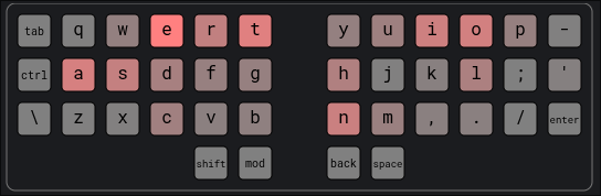
2. My chosen handsdown-promethium layout:

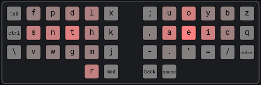
So, not only did I have to adjust to a new keyboard shape, but also to a completely new key layout. Yes, it was brutal, painfully difficult at first.

That said, I’m very happy with handsdown-promethium. Honestly, I think almost any modern layout is a huge step up from QWERTY. This site provides useful statistics on different layouts to back that up. For example, QWERTY’s Total Word Effort is 2070.6 while handsdown-promethium is only 763.5.

Programmability and Practice

One of the Glove80’s best features is its programmability. I could remap keys, add layers, and customize shortcuts directly on the keyboard. These three features make it possible to tailor the keyboard to my workflow instead of forcing myself to adapt to it.

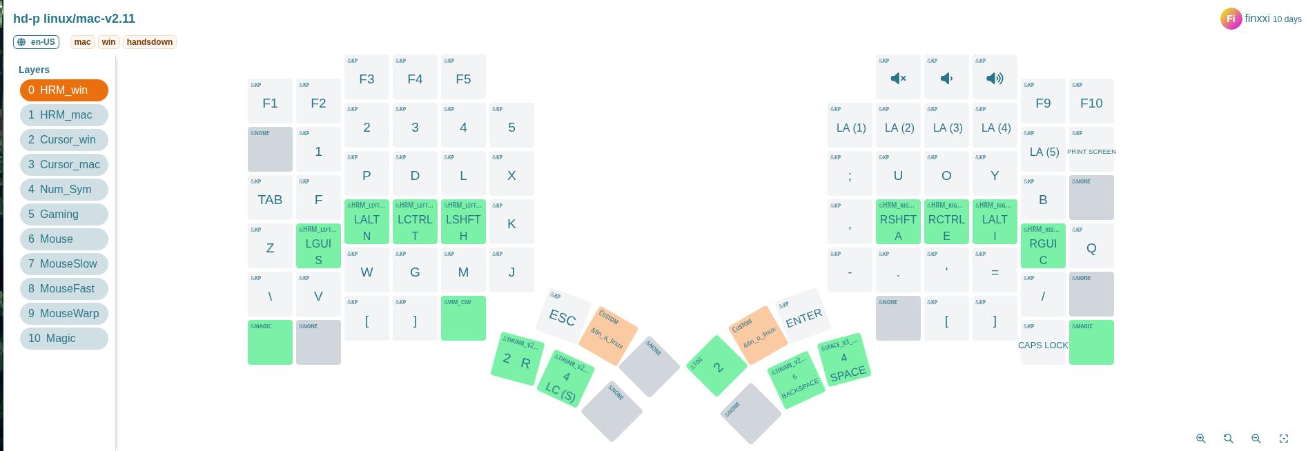
Layers

A layer is like having multiple keyboards in one. Your base layer handles normal typing, but with a single key press you can switch to another layer—for numbers, symbols, navigation, or anything else. On the Glove80, I set up separate layers for symbols, numbers, cursor movement, and even mouse control. With cursor keys and mouse emulation built in, I rarely reach for an actual mouse—especially when using a tiling window manager like Hyperland.

Home Row Mods (HRM)

Another powerful feature is Home Row Mods. With HRM, keys on the home row act as normal letters when tapped, but as modifiers (Ctrl, Alt, Shift, etc.) when held.

In my case, s, n, t, h on left hand and a, e, i, c on righe hand are my modifiers as shown on the glove80-layouts screenshot above.

This means I don’t need to stretch my fingers awkwardly to reach modifier keys, reducing strain and speeding up key combos.

The Practice Phase

The first few weeks were slow. I had to retrain my muscle memory while learning both a new keyboard shape and a new layout. Daily practice on keybr.com was essential. Gradually, my typing speed and accuracy started to recover.

Integrating Into My Workflow

Once typing felt natural again, the next step was adapting my dotfiles and tools. For me, that especially meant reconfiguring Tmux and Neovim to fit the new layout. Even small adjustments made a big difference in keeping my workflow smooth and efficient.

One challenge of using a non-QWERTY layout is Vim’s navigation keys. Traditionally, h, j, k, and l sit comfortably on the home row, making them ideal for movement. On Handsdown-Promethium, however, these keys are no longer in the same resting positions, so an alternative was needed.

My solution was to rely on the arrow keys in a dedicated cursor layer. On the Glove80, they map neatly to the same physical positions as hjkl on a standard keyboard, which makes the transition more natural. At the same time, Handsdown-Promethium still places hjkl in reasonably accessible spots, so I can fall back on them if I want.

This hybrid approach has worked well: I get the familiarity of Vim-style navigation without forcing my fingers into awkward positions.

Typing Demo

Here’s a 1.5-minute typing demo ~40 WPM (words per min) recorded on 13-09-2025.

Notes:

• The printed letters on the keycaps are QWERTY, so they don’t match my actual layout.
• Finger and hand movement is very minimal, which shows the ergonomic advantage.

Final Thoughts

Switching from the Sculpt to the Glove80—while also changing layouts—was not easy. The transition took multiple weeks of patience and practice.

But now, three months later, typing feels lighter, smoother, and more sustainable. I no longer feel the same tension in my shoulders and hands.

If you spend hours typing each day, investing in both an ergonomic keyboard and a better layout is worth it. The short-term pain pays off in long-term comfort and efficiency.

Salesforce Developer Training

This training aims to coach general software engineering skills for Salesforce developers so they can deal with large solutions in the long run.

The Issue it solves

Salesforce platform is a sizable business investment. However, many solutions deteriorate after the first several years.

New features take too long to publish, bugs appear here and there. This issue is actively discussed on LinkedIn: video1, video2

It won’t fix the problem by throwing more developers or testers. On the contrary, a small dev team with the right software engineering skills can manage large solutions.

Content

This training aims to coach the essential software engineering skills for your development team.

The training is one or two days, and include subjects like:

• Clean code concept
• Object Oriented mindset
• Separation of concerns concept
• Unit testing practice and tooling
• Refactoring code
• Salesforce modularization
• Salesforce DevOps

After the training the participants will be able to:

• Understand how to structure the code
• Understand and use clean code concept in work
• Create Object Oriented code in Apex
• Know what is unit testing and how it helps code refactoring
• Know cutting-edge Salesforce 2nd gen package and modularization
• Modern DevOps tools in Salesforce

Requirement

This training requires active participation in discussions and frequent small hands-on Apex programming exercises.

This training can be customized according the your dev team skill level. Follow up and feedback sessions after the training are also highly recommended

To book the training, contact me at tdxiaoxi2@gmail.com.

Thanks for your time!